Expert Excel Help: Pivot Tables for Summarizing data-sets
Recently, we demonstrated how to use the sophisticated SUMIF function to extract data from large data-sets, see previous blog. We also mentioned that there is a more straight forward way to achieve a similar result in Microsoft Excel 2010 by using a Pivot Table. So let's look again at the same data set and see how Pivot Tables can be used.
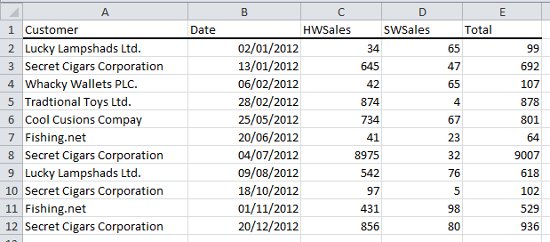
Once again we have a list of software and hardware sales from companies with multiple entries for some companies. Creating a Pivot Table from some or all of the data is simple.
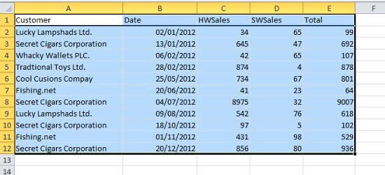
First of all, simply select the data you would like to use - in this case we are selecting all eleven rows of data representing sales for 2012, but you could select thousands of rows if necessary.
We then simply go to the menu bar and click on Insert and then in the Tables options we click on the PivotTable icon. A box appears confirming the data range and asking us where we would like the table to appear.
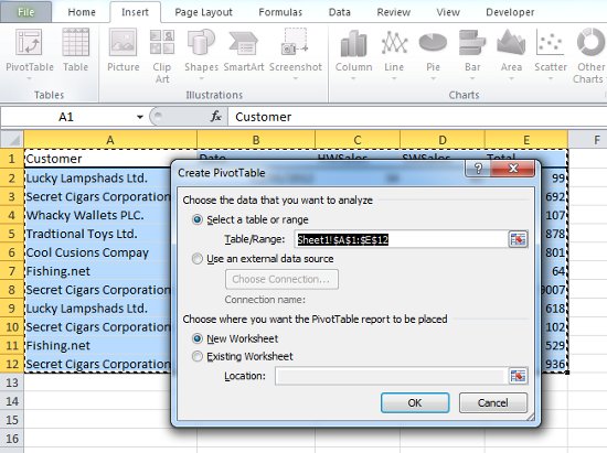
In this case we will simply click OK and the table will appear in a new worksheet.
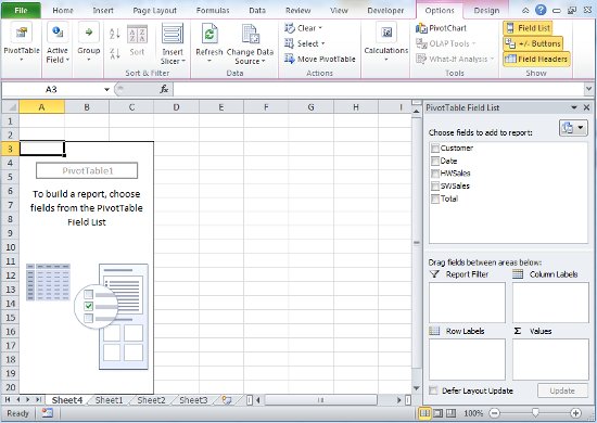
At this stage our table has no data. On the right hand side we can select the summarized data we would like. For example, if we select the Customers check box, a summary of our customers will appear. Likewise, we can select the SWSales, HWSales or Total sales and they will immediately be associated to their customers.
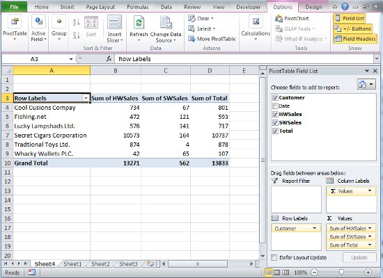
We now have a quick and convenient way to summarize individual or related elements from my original data set. For more details and ideas on how to use Pivot Tables, see the Microsoft website.


