Excel Formula Help - A Simple Introduction to CSE Array Formulas
First of all, these Microsoft Excel CSE array formulas are not difficult. In this example, the concept is similar to COUNTIF and SUMIF; So, if you understand those functions, then understanding this blog is easily within your reach.
CSE stands for Control-Shift-Enter, which are the keys you need to press in order to get the result of your formula. Just hitting return will usually give you the less than useful error code, # VALUE!.
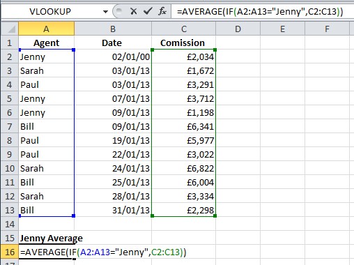
Let's look at some data. In this example there are 4 Estate Agents who each record their commission throughout the month. At the end of the month, we wish to know the average commission each Agent achieved per sale. Entering the =AVERAGE(IF(A2:A13="Jenny",C2:C13)) formula in A16 will provide our answer:

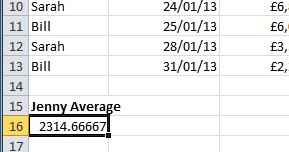
Notice the similarity to the SUMIF and COUNTIF functions, both of which are derived from CSE formulas. Importantly, we now need to activate the CSE formula by holding down Ctrl and Shift and then pressing Return. For Jenny, we now have an accurate average of £2314 in cell A16, once we correctly format the cell.

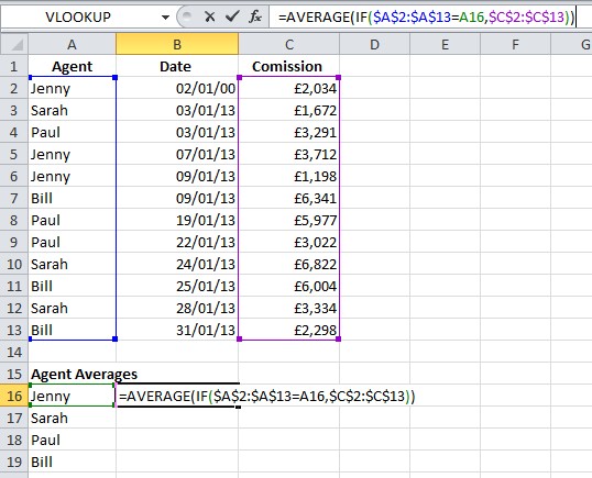
To be able to copy down the formula, we need to specify the Value of the contents of A16 (now the Agent name, below) and then add absolute references in the form of $ symbols to our coordinates (see this blog from more about absolute references). Our final formula entry, now moved to B16 should be: =AVERAGE(IF(A$2$:A$13$=A16,C$2$:C$13$)), as seen here:

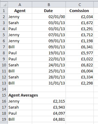
We can then copy down the formula in the normal way to produce our final average figures:

For more help with CSE formulas, contact our experts or visit the Microsoft Help pages here.


