Excel Formula Help – Nested IFERROR statements with VLOOKUP for searching through multiple sheets
Searching through multiple Microsoft Excel sheets for specific data is straight forward. In this blog, we will look at an example using both the IFERROR and VLOOKUP functions.
IFERROR works similar to an IF statement, however it 'Returns a value you specify if a formula evaluates to an error; otherwise, [it] returns the result of the formula.' In summary, we 'Use the IFERROR function to trap and handle errors in a formula.' (Microsoft Excel Help pages)
VLOOKUP has been covered before in these pages; for a reminder of how it works you may familiarise yourself here and here.
Our example will cover the ability to use an employee number to search through multiple Excel sheets to find the name of that employee. Furthermore, if no number/employee combination is found, the formula with return with a Not Found notification.
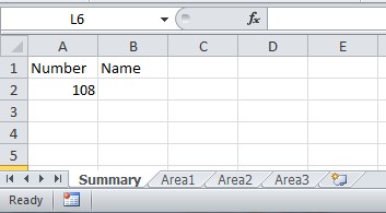
Let's look at our worksheets, beginning with the Summary sheet where we enter the employee number we wish to search.
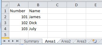
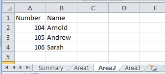
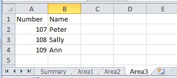
As we can see, there are further sheets covering 3 Areas:
To begin, we firstly, we select the location for our formula result, cell B22. Using the sequence, =IFERROR(value,value _ if _ error) we include VLOOKUP as the value, which, by default, will search the present sheet. We then we define the lookup, first the lookup _ value - the contents of A2; then table _ array; then column _ index _ num - the column than contains the actual values we wish to return (the employee names); finally we use FALSE to tell excel that we need an exact match:
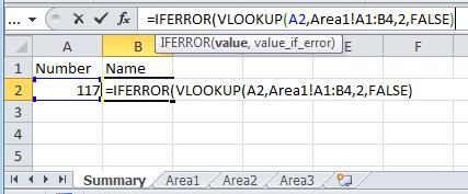
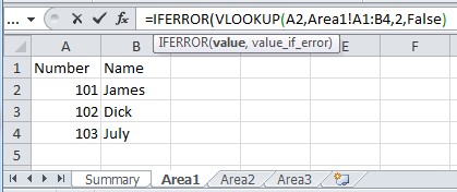
The formula is now directed to search through the Area1 sheet.
What we can see if we look closely is that we have also defined the sheet name as a part of the table_array value. This is the key to using multiple sheets and is added simply be clicking on the required sheet after we have selected the lookup _ value. Once this is done, we use a comma and essentially start the process again to add further sheets. Importantly, this time we need to specify in the formula where the lookup _ value is, in this case on the Summary sheet.

We do this in the same way that we specified Area1 in the first nested IFERROR syntax. The formula will now be capable of searching through the Area2 sheet.
Finally, we need to add the final repeated syntax which will include Area3 in the search. Be careful to ensure that each syntax chunk is separated by a comma with no spaces. Following the last chunk, and a comma, we add in quotation marks, Not Found, which tells the formula to return this value is no lookup match if discovered. We close the formula with three closing brackets relating to the three opened IFERROR functions:

The image here is very small, so the complete formula is written out here:
=IFERROR(VLOOKUP(A2,Area1!A1:B4,2,FALSE),IFERROR(VLOOKUP(Summary!A2,Area2! A1:B4,2,FALSE),IFERROR(VLOOKUP(Summary!A2,Area3!A1:B4,2,FALSE),"Not Found")))
We are now ready to test our formula. Entering 108 returns Sally and 105, Andrew:
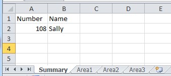
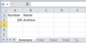
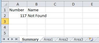
All good so far; And if we try to search for a number that is not on the system, we receive our programmed Not Found result.
For more help and advice with Excel formulas of all kinds, contact our Experts. Specific details on IFERROR can also be found on the Microsoft Excel Help page, here.


